Here is a very quick and basic note on how linearity in features can be used to find the best-fitting polynomial. This is a trivial corollary to how linear models are set up, but for some reason most uni classes focus on fitting a literal line, which seems a bit underwhelming. So suppose something is related as a quadratic. Let's say this "hidden" relation is $f$ defined as follows
f <- function(x) {
  2 * x^2 + 3 * x - 10
}
Now, suppose we can gather 50 points observed with some noise. Native vectorization in R makes our life easy.
n <- 50
x <- 1:n
y <- f(x) + rnorm(n, sd = n)
data <- data.frame(x = x, y = y)
Define our model with another nifty R expression and hope for the best.
model <- lm(y ~ x + I(x^2), data)
summary(model)$r.squared > 0.9 # Most likely true
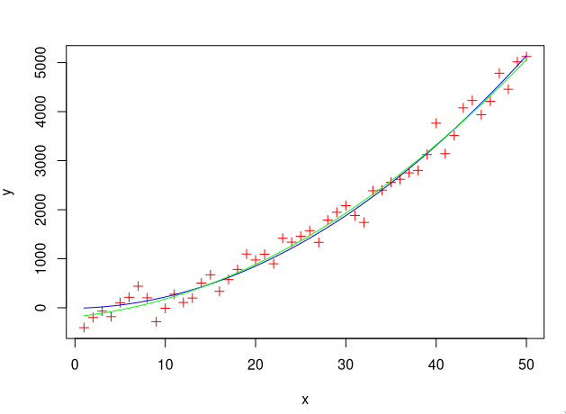
Nice! Let's also see how well did we do on a plot. We recover the fitted polynomial from the model coefficients and plot the points in red, original map in blue and our fitted solution in green.
g <- function(x) {
  model$co[3] * x^2 + model$co[2] * x + model$co[1]
}

plot(data, pch = 3, col = "red")
lines(1:n, f(1:n), col = "blue")
lines(1:n, g(1:n), col = "green")
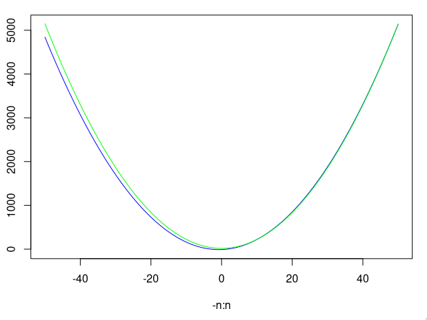
We even get a decent fit on the unseen data with just 50 points (but only because polynomials and normal noise are so nice).
plot(-n:n, f(-n:n), type = "l", col = "blue")
lines(-n:n, g(-n:n), col = "green")
Voila :)
01 February, 2020